This Landscape Does not Exist: Generating Realistic Landscape Imagery with StyleGAN2
Out of college I worked for a GIS+AI company which taught me a lot about how startups can fail1. It also gave me a lot of exposure to remote sensing imagery, which turns out to be pretty interesting and fun to work with! I originally wrote this post in 2021 shortly after leaving, and since I’ve made a new blog I’m reposting it here in it’s entirety2. GANs aren’t really popular anymore now that we have transformers and diffusion models, but I still really liked this project and think it’s interesting to read abut.
Motivation
GANs can generate staggeringly realistic outputs. This Person Does Not Exist showcases Nvidia’s StyleGAN2 which generates portraits of people who, as the name suggests, do not exist — and with uncanny realism. Sadly for the hobbyist, training state-of-the-art networks typically requires a huge amount of compute resources and massive amounts of data. The first implementation of StyleGAN took more than 41 days to fully train and required 8 Tesla V100 GPUs. And that doesn’t even include the hyperparameter search!
Late last year, an improvement to the augmentation mechanism of StyleGAN2 called Adaptive Discriminator Augmentation was released, which supposedly stabilizes training on smaller datasets. This piqued my interest: would it be possible to train a network like StyleGAN2 using only resources that were freely available to me? Looking a bit deeper, it seemed possible, so I decided to dive in head-first.
Generating a Dataset
There exist plenty of publicly-available image datasets which can be used to train networks like StyleGAN2. But since this project was an experiment, I thought it would be more fun and interesting to build something novel. I have experience in the GIS industry, and chose to leverage this to create a large-scale dataset of remote sensing imagery (i.e. satellite photography). This essentially means that I would gather a bunch of images that look like the stuff you see on Google Earth — overhead views of forests, lakes, cities, etc. Everyone has fun poking around satellite or aerial imagery on Google Earth; with any luck, it would also be fun to poke around the outputs of my trained model!
How much data would I need? The paper published by the authors of StyleGAN2 describes two fully-trained models, one which generates images of human faces and another which generates images of cars. The datasets on which these models were trained contain 70,000 and 893,000 images respectively. FFHQ, the dataset containing faces, is more structured and consistent than the car dataset, LSUN Car. Because of this structure, the target distribution which StyleGAN was trained to approximate is narrower for FFHQ than for LSUN Car. This allowed the face model to generalize with fewer training examples. In order to achieve comparable results, my dataset would need somewhere around 100,000 images that fall into a narrow domain. This means a large volume of consistent data needed to be sourced.
Sourcing Imagery
Finding a reliable source for high-quality imagery was actually the most time-consuming part of this project. I went down a number of paths before settling on one that felt worth following to the end.
There are lots of sources for free remote sensing data available online. My first approach was to use imagery from Landsat 8, a satellite developed by NASA with a moderate-resolution multispectral sensor (i.e. each pixel is about 15 meters wide). The Landsat program surveys nearly the entire world, which makes it an attractive option for creating a large-scale dataset of overhead imagery. After downloading a section of data with USGS’s Earth Explorer, however, I ran into a couple contingencies:
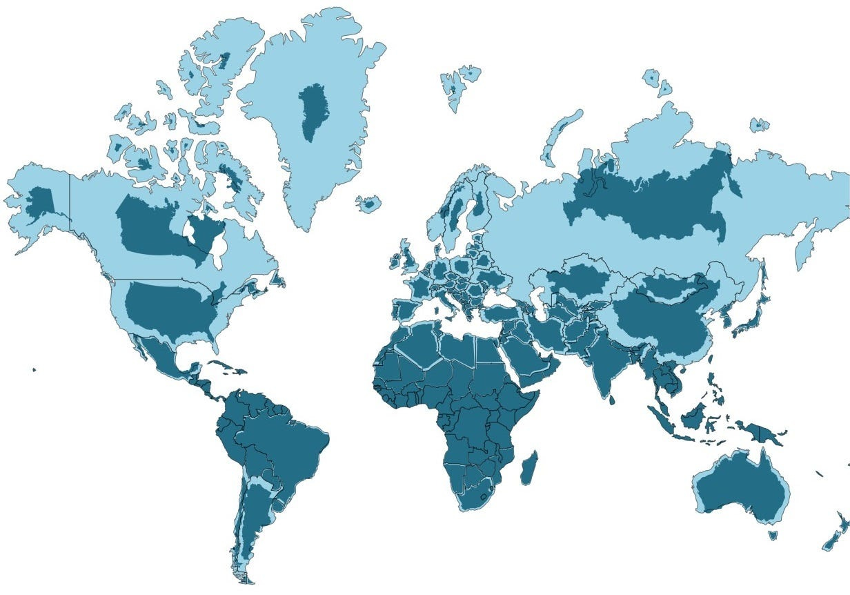
1. Images are flat, but the Earth is not. Landsat imagery is provided using the Mercator projection, which translates coordinates on a globe to a Cartesian grid. This is great for a lot of applications, but introduces an artifact where features close to the equator appear much smaller than features far from the equator. Without correcting for this, the full dataset is less homogeneous, forcing a model to learn a wider output distribution and increasing the likelihood of overfitting.

2. Most of the world is just not that interesting from far away.
These problems are both solvable, but in the spirit of experimentation I decided to keep looking around.
Something caught my eye when browsing data on USGS’s platform: they provide a very high resolution base map on their map viewer, which has a maximum resolution around 50x sharper that of Landsat 8. With such high resolution imagery, a smaller geographical area could be sampled and there would be no need to correct for projection distortion. Better yet, multitudes of interesting man-made structures are clearly visible at the maximum zoom level. EarthExplorer doesn’t provide an option to directly download this data, but taking a peak at Chrome’s developer tools reveals a URL for the imagery:
With this URL and some google searching, an endpoint designated for export which required only a free ArcGIS developer account was revealed. Nice!
Now that I had high resolution imagery to work with which can be loaded into a GIS tool, I found an interesting looking region in Italy and exported it as a set of 512x512 pixel PNG tiles. I chose an area surrounding Rome which looked fairly homogeneous but also had some interesting features, like vineyards, farm land, small villages, and large towns. This yielded around 280,000 images.
Preparing the Dataset
The map provided by ArcGIS was already very high quality, so minimal dataset cleaning needed to be done. I ended up filtering out images containing no data (high-res imagery was not available for the entire region), and images containing only water. This was done with a simple python script:
for i, file in enumerate(os.listdir(tiles_dir)):
    file_path = os.path.join(tiles_dir, file)
    img = cv2.imread(file_path)
    if img.std() < 6 or img.std() < 20 and img[:,:,1].sum()/(512**2) < 42:
        shutil.move(file_path, os.path.join(filtered_dir, file))
The first check, img.std() < 6, filters out images which contain no information and were exported as a pure gray raster with some text. The second check, img.std() < 20 and img[:,:,1].sum()/(512**2) < 42, filters out low-information imagery with small average intensity values on the green channel. This was tuned to exclusively and almost entirely detect images of the sea, which would not have been interesting to model.
The full dataset contains just under 200,000 images after cleaning, more than enough to train a network!
Nvidia provides a useful script dataset_tool.py which converts images into .tfrecords. After running this and uploading the dataset to a newly spun-up GCP compute instance, the model was ready to be trained.
Training
The authors of StyleGAN2 originally trained the FFHQ model on 8 Tesla V100 GPUs for 9 days and 18 hours. This figure is for a single training run, and does not include a hyperparameter search. Regrettably, I do not have 8 Tesla V100 GPUs nor did I want to spend ~$4,600.00 to provision them on Google Cloud Platform. I did, however, have access to $300 of free credits allotted to new GCP accounts, which was enough to spin up a single V100 cloud instance for a bit under 5 days. Even though I had less than 1/10th the compute the researchers used, I figured I could still get some decent looking results for a couple reasons:
Training could be done on smaller images, reducing the size of the network and increasing training speed
Training could be stopped early before the loss had fully converged
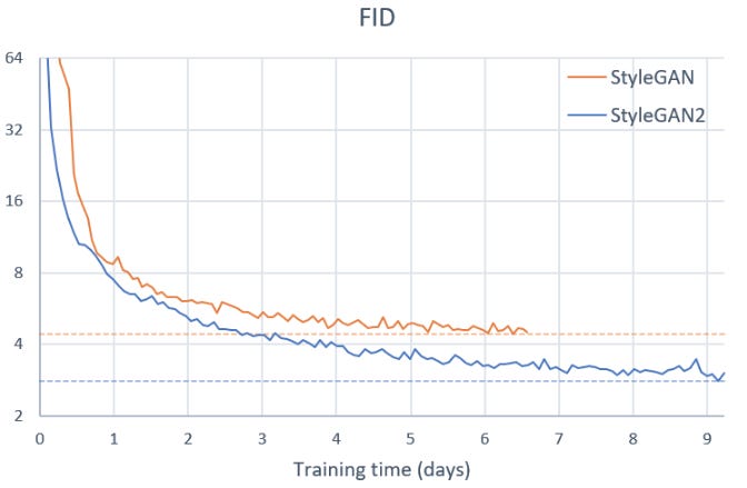
Using 512*512 pixel images instead of the 1024*1024 images that were used in the paper theoretically allows a model to see four times as many images during training using the same amount of GPU memory. Given the constraints, this seems like worthwhile compromise. Taking a look at training curves from the official StyleGAN2 repository on GitHub, it can be seen that most of the performance gains happen within the first few days of training, while in the remaining days performance gains begin to plateau. Some very cursory back-of-the-envelope math can approximate the performance one can expect with this paradigm:
5 training days * (1 GPU/8 GPUS) * (4 images/1 image) = 2.5 training days
This is to be taken with a gigantic grain of salt, but the approximation suggests that with smaller images and fewer GPUs, similar performance to what the original authors achieved after ~2.5 days of training can be expected. Taking another look at the published training curves, it looks like training for the equivalent of 2.5 days should yield some interesting results.

In reality, there are many confounding factors which affect training speed. It’s unlikely that training speed scales linearly with image size, and multi-GPU training utilizes larger batch sizes and thus larger or more precise training steps which affect the path taken during gradient descent. Still, this is a useful sanity check which validates the approach, and indicates that the expected performance of the model should be somewhere around “not bad”.
Results
The actual process of developing this dataset and training this model was a lot less straightforward or contiguous than this blog post makes it out to have been. I had played around with some other data sources, tried out different image resolutions, and even experimented with false color composite imagery. After working out some bugs and false starts, I had a bit over two and a half days of compute left to train the final model. Not quite what I had planned for, but hopefully still enough to get some strong results.
Again plotting FID against time, it can be seen that model performance was beginning to converge by the time training stopped. This is good news, as it means that there likely wasn’t a huge amount of performance lost from cutting off training early.
The final FID was slightly above 12.05. This is a bit higher than I was expecting after extrapolating from Nvidia’s results on various datasets, and could be due to an underfit network or the dataset being hard to model. Because of the resource limitations I was working with, I couldn’t perform a robust hyperparameter search and had to resort to using the default configuration which was provided by researchers (this seemed to work reasonably well). Though a better performing model could be trained with a more thorough search, I feel that the results are quite satisfying:
This video was rendered by sampling points randomly from the input distribution, interpolating them using SciPy’s implementation of cubic spline interpolation, and feeding them into the network.
While fun to watch, this interpolation video also reveals some interesting information about the trained model. It appears the model is not overfit; nearly every frame in the video looks like a valid landscape, and the model is not jumping from memorized output to memorized output. The smooth transitions from point to point suggest that the model is successfully generating new and diverse images, and is not suffering from mode collapse.
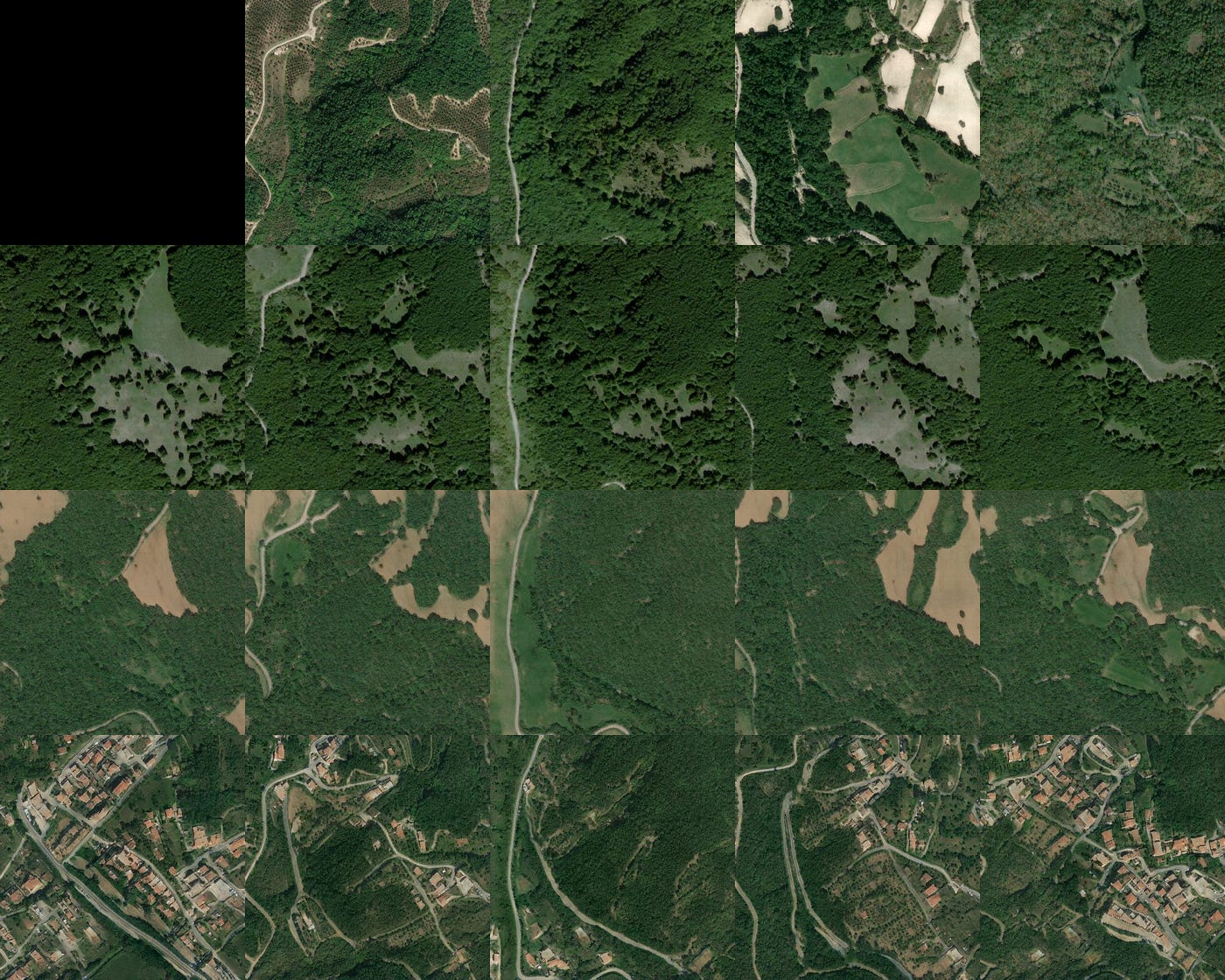
Also interesting is the following visualization of something SytleGAN’s authors call style mixing. Style mixing is the practice of feeding in different latent vectors to different style blocks during inference. StyleGAN2 has multiple style blocks which each correspond to a different level of abstraction, meaning it is possible to alter low-level features of the image (e.g. geographical features or topography) without modifying high-level features (e.g. presence of trees, buildings, roads, etc.), or vice versa. A matrix of images can be generated where low-level features are held constant for each column, and high level features are held constant for each row:

Reflections
Musings on Future Work
If I were to do this again, I’d probably spend more effort optimizing time spent with the expensive V100 instance. The GPU was only running ~80% of the time, the remaining 20% was spent on data processing that could have been done offline. I’d love to see how more training time, or even a hyperparameter search, would improve the model’s outputs.
It would be interesting to try to isolate human-interpretable features from the 512-dimensional latent space, perhaps with principal component analysis. Nvidia has isolated features for age, hair color, face-direction, etc. I’m curious to see what features emerge from my model.
Some kind of framework for spatial interpolation would be particularly interesting. When viewing a map on your phone, you don’t view a grid of discontinuous images, but rather a mosaic that appears to be one large image of the Earth’s surface. Recurrent neural networks may be able to achieve something like this, though integrating RNNs with a GAN architecture is sure to be non-trivial.
Final Thoughts
I’m pretty happy with the way everything turned out. It was a fun project to work on, and I’ve reached my goal: proving that it’s possible to achieve reasonable performance on (certain) state-of-the-art networks with a novel dataset and limited compute resources. I’ve also gotten a lot of positive reactions from people watching the interpolation video, even without a technical background — there seems to be something universally mesmerizing about it, which is a quality of machine learning that gets me really excited.
It was actually a good experience and I worked with some great people — we just couldn’t make it work.
*except part of the intro which I removed because my old writing makes me cringe :)


